Cost benefit analysis template excel

Cost benefit analysis template excel

Free Cost benefit analysis template excel

Cost–benefit analysis (CBA), sometimes also called benefit–cost analysis, is a systematic approach to estimating the strengths and weaknesses of alternatives used to determine options which provide the best approach to achieving benefits while preserving savings (for example, in transactions, activities, and functional business requirements).

A CBA may be used to compare completed or potential courses of actions, or to estimate (or evaluate) the value against the cost of a decision, project, or policy. It is commonly used in commercial transactions, business or policy decisions (particularly public policy), and project investments. For example, the U.S. Securities and Exchange Commission has to conduct cost-benefit analysis before instituting regulations or de-regulations.

Conventions used in the Cost Benefit Analysis (CBA) Toolkit:

1. The CBA Toolkit is an Excel Workbook containing five worksheets:

• Summary 
• Do Nothing 
• Alternative 
• Alt 1 
• Alt 2 
• Alt 3

2. Each worksheet contains locked cells.  Those cells without color or gray are unlocked and indicate where data input is required.  Cells with color or gray indicate those cells that are locked and cannot be edited. 

• The password to unlock is: "CBA"

3. Data entered into last four worksheets (Do Nothing, Alt 1., Alt 2., Alt 3.) are used for calculations in the first worksheet, Summary.

Instructions for Completing CBA Calculations:

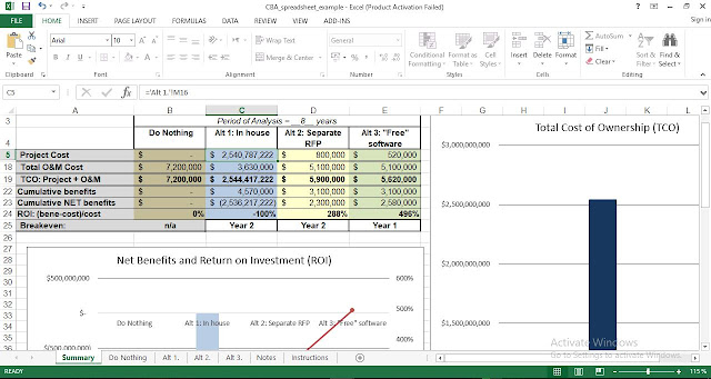
Go to the spreadsheet tab Summary:

1. Cell C1: Enter the name of the Project b 
2. Cell 83: Enter in the period of analysis
• Note: The Project Management Standard requires six years of O&M analysis once the new product/system is implemented.
• Note: Since it might require 1, 2. 3 years or more to implement the new product/system, the six year O&M analysis begins upon implementation. 
• In the example. it took two years to implement the new system, thus the period of analysis is eight years (2 + 6 = 8).
3. Cell C4: Alt 1. Enter in very brief name of Alternative 1. 
4. Cell D4: Alt 2. Enter in very brief name of Alternative 2. 
5. Cell E4: Alt 3. Enter in very brief name of Alternative 3, if needed. 
6. The values presented are calculated in the last four worksheets and are re-presented here and cannot be edited in the Summary tab. 
7. Note that you can Unhide rows 6-18 and 21-22 if you wish. These also are values simply re-presented from the last four worksheets and cannot be edited in the Summary tab.

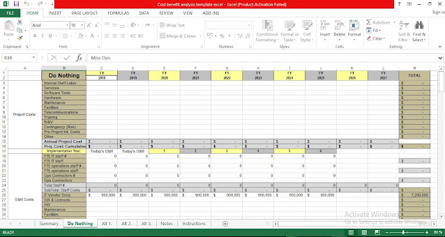
Go to the spreadsheet tab Do Nothing:

1. This tab represents 
1. the current cost of owning and operating the current. legacy system, and
2. the estimated cost of continuing to use the current, legacy system for the period of time it takes to implement Alternative 1, 2 or 3, plus six years. 
2. Cell C2: Enter in the first year (fiscal year (FY)) of analysis; the subsequent years will automatically populate. and all three Alternative tabs automatically populate. too. 

Costs: 

1. Rows 3-16: Project Costs: There are NO project costs in the 'Do Nothing' scenario. 
2. Rows 18-37: O&M Costs: As follows: 
3. Row 17: Adjust (using Copy & Paste) implementation year(s) and six years of O&M. Make sure all three Alternatives match the Do Nothing tab to ensure equivalent comparison.
4. Note that the annual. (row 35) cumulative (row 36) and total (column M) O&M costs are calculated. 
5. Note that the cumulative (row 37) and total (column M) Total Cost of Ownership (TCO) (project + O&M costs) are calculated. 

Benefits:

1. Row 40: Move the six years of analysis (using Copy & Past) left or right to match the Do Nothing Tab. Make sure all three Alternatives match the Do Nothing tab to ensure equivalent comparison. 
2. Benefit 1.: <calculated field> : Cost Savings: O&M savings compared to "Do Nothing" alternative ("Do Nothing" row 35 - row 35) i. Note: For the to Nothing° scenario, there is no O&M savings to report. thus this value should be zero. I. Benefit 2.: Cost Avoidance: If we select this alternative, we will AVOID certain costs associated with the to Nothing' scenario. i. Note: For the To Nothing" scenario. this value should be zero. 
3. Benefit 3.: Increased Revenues: If we select this alternative. our organization will collect additional revenues. compared to "Do Nothing". i. Note: For the to Nothing' scenario. there likely is no additional revenues savings to report, thus this value should be zero. 
4. Benefit 4.. Other cost savings. cost avoidance or increased revenues. Explain the savings and the calculations. 
5. Benefit 5.: Other cost savings, cost avoidance or increased revenues. Explain the savings and the calculations. 
6. Note the cumulative Return on Investment (ROI) is calculated. R01=(benefit - project cost)/project cost 
7. Note that the breakeven year can be determined where the ROI changes from a negative % to a positive %.

For Alternatives 1. 2 and 3 (tab Alt 1.. Alt 2.. 611.2j: 

1. Each Alt tab represents an alternative solution to the business problem presented in the BCAA. 
2. Cell C2: The first year (fiscal year (FY)) of analysis will automatically populate from the To Nothing' first year. Subsequent years will also populate. 

Costs: 

1. Rows 3-16: Project Costs: Enter costs to implement the project. 
• These figures are estimates: additional justification/explanation can be entered into BCAA. 
• Note: These figures can be copied and pasted directly into CTP project budget forms 
2. Rows 18-37: O&M Costs: As follows: 
3. Row 17: Make sure all three Alternatives match the Do Nothing tab to ensure equivalent comparison. f. Rows 18-23: Staff Costs: Enter the number of (a) FTE IT staff. (b) FTE operations staff, and (c) Operations Contractors and the annual cost for each.
• These figures represent additional staff. above current staffing level. 
• If the solution results in fewer staff. those savings should be listed in Benefit 4 or 5 and explained. 
• These are estimates; additional justification/explanation can be entered into BCAA.
4. Rows 26-34: Enter in the O&M Costs. i. These are kill-cost estimates; (not the difference compared with today) additional justification/explanation can be entered into BCAA. 
5. Note that the annual, (row 35) cumulative (row 36) and total (column M) O&M costs are calculated. 
6. Note that the cumulative (row 37) and total (column M) Total Cost of Ownership (TCO) (project + O&M costs) are calculated. 

Benefits: 

1. Row 40: Move the six years of analysis (using Copy & Past) left or right to match the Do Nothing Tab. Make sure all three Alternatives match the Do Nothing tab to ensure equivalent comparison. 
2. Benefit 1.: <calculated field> : Cost Savings: O&M savings compared to "Do Nothing" alternative ("Do Nothing" row 35 - row 35) 
• Note: A positive value indicates a cost savings: a negative value indicates comparatively increased costs. 
3. Benefit 2.: Cost Avoidance: Cost Avoidance: If we select this alternative. we will NOT have to purchase in the "Do Nothing" scenario. 
4. Benefit 3.: Increased Revenues: If we select this alternative, our organization will collect additional revenues. compared to "Do Nothing". 
5. Benefit 4.: Other cost savings, cost avoidance or increased revenues. Explain the savings and the calculations. 
6. Benefit 5.: Other cost savings, cost avoidance or increased revenues. Explain the savings and the calculations. 
7. Note the cumulative Return on Investment (ROI) is calculated. R01=(benefit - project cost)/project cost q. Note that the breakeven year can be determined where the ROI changes from a negative % to a positive %.

Note: When pasting from CBA.xlsx into CTP. CTP does not handle ($ - ) very well. Instead of keying in zero into the CBA cell, just leave it blank. That should allow you to copy from CBA into CTP without a problem.

Note: The password to unlock cells is: CBA.

Download also:

• Project Status Report Excel Template
• Change Management Log Template
• Procurement Schedule Template Excel
• Risk Management Tracker Template in Excel